Computing fractal images
This page briefly describes the techniques used by the app for rendering fractals images (including some basic maths). You may find it useful for defining your custom fractal types and paint modes, or for writing your own computer program creating fractal images.
You should be able to use the app without reading this page. 😃
Rendering escape-time fractal image
A fractal image is rendered by assigning to each pixel a color calculated based on its coordinates (x, y) and a given fractal formula.
A pixel coordinates can be treated as the real and imaginary parts of a complex number. This number is called current point coordinates (or simply: current point) and is denoted by c.
Escape-time fractals are computed by repeatedly applying a given formula, starting from the arbitrarily chosen initial value z0, until the specified escape conditions is met.
The classic Mandelbrot Set fractal uses z2+c formula and is defined as follows:
z0 = 0
zi+1 = zi2 + c
The subsequent values of zi are calculated until the absolute value |zi| exceeds the chosen threshold value (called bailout) or the iteration count reaches the chosen limit (called iteration limit).
The key aspect is to refer to the current point c in the fractal formula (or in the initial value definition) which causes the results to differ from point to point.
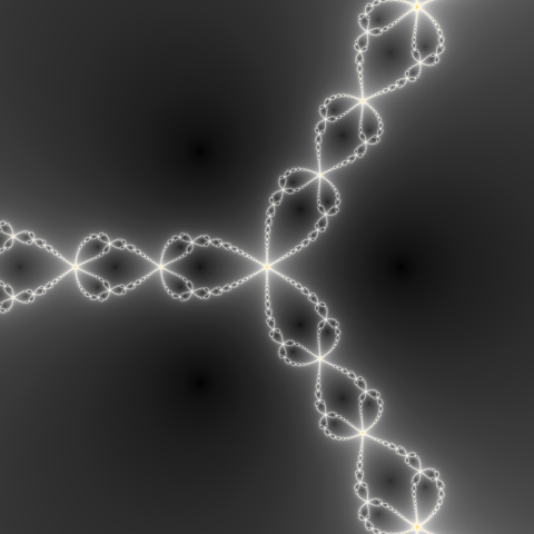
The simplest rule for assigning a color to a pixel is: black for the pixels where computing stops due to reaching the iteration limit (which means that the pixel belongs to the Mandelbrot Set), and white for the pixels where it stops due to exceeding the bailout value.
The area where the bailout value has been exceeded is called fractal exterior or bailout area. The are where the iteration limit has been exceeded is called fractal interior or lake area.
A more formal explanation can be found here.
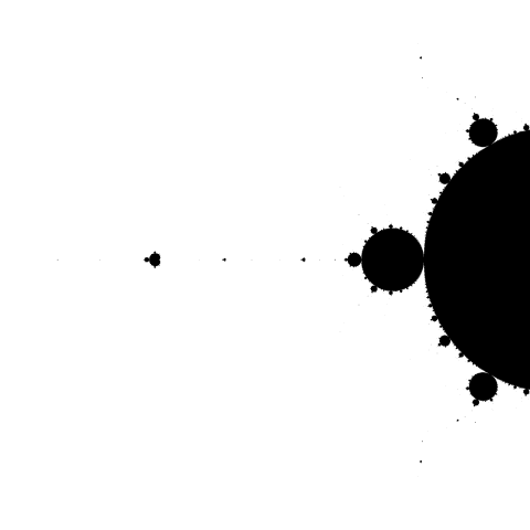
The Mandelbrot Set left antenna image colored black (interior) and white (exterior).
The following sections describe the whole process in more detail, including using various escape conditions and various coloring techniques.
Mapping pixels to coordinates
Let's assume that we want to render a square image of size s=100 (in pixels) for the actual coordinates (x0, y0) = (-0.7625, -0.0895) and zoom factor of 500.
The central pixel image coordinates are (xc, yc) = (50, 50) in pixels. These image coordinates should correspond with the actual coordinates (x0, y0).
Suppose that at zoom=1 the image should cover the area of the actual size 1 (width and height). So at zoom=500 the actual image size is
1 / zoom = 0.002
and the distance between adjacent pixels is
(1 / zoom) / s = 0.00002
So for the pixel of image coordinates (xi, yi) we should perform the calculation for the following actual coordinates:
x = x0 + (xi - xc) * (1 / zoom / s)
y = y0 + (yi - yc) * (1 / zoom / s)
For the example image size, coordinates and zoom factor we have:
x = -0.7625 + (xi - 50) * 0.00002
y = -0.0895 + (yi - 50) * 0.00002
Actually, the app uses a viewport size of 4 which means that at zoom=1 and coordinates=(0, 0) the image covers the area with the corners in (-2, -2) and (2, 2). This is for the backward compatibility with the very first version of the app computing only the Mandelbrot Set which fits that area.
Divergence escape
As the result of computing for given coordinates we get a sequence of n complex numbers:
z0, z1, z2, z2, ... , zn-1
which is called orbit. The orbit length n is bounded by the iteration limit.
The following chart shows two example orbits for the Mandelbrot Set. The blue one is for the point (0.25, -0.4) and the red is for (-1, 0.31).
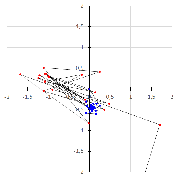
Example Mandelbrot Set orbits.
The blue orbit keeps bounded which means that the current point belongs to the Mandelbrot Set.
Some initial elements of the red orbit remain limited, but then the absolute values go high, never to return. We call such an orbit divergent. In this case, the current point does not belong to the Mandelbrot Set.
For the Mandelbrot Set, it was proved that when the element absolute value exceeds 2, the orbit will diverge.
For the most-used escape-time fractal formulas based on polynomials, the orbit keeps bounded within a limited area (called fractal interior or lake area) and diverges outside (in the area called fractal exterior or bailout area).
The key to rendering fractal images is detecting whether a certain point belongs to a fractal interior or not. The simplest way is to stop the iteration when the absolute value exceeds the arbitrarily chosen value (called bailout). When the iteration stops due to exceeding the bailout value, we treat the current point as a part of the fractal exterior.
The app's built-in DIVERGENCE escape condition is defined as follows:
rad2 z >= bailout
Note that the squared absolute value |z|2 is used. This is because computing |z|2 is faster (you avoid calculating the square root).
|x + i y|2 = x2 + y2
The bailout value used for the simple fractal definition is 2e+8. You may change it using the advanced definition.
For the Mandelbrot Set, the bailout value of 4 is sufficient but using higher values results in better smoothing.
Root-finding fractals (convergence escape)
Root-finding fractals are generated by applying a root-finding algorithm for a given function using the current point as an initial guess.
For example for the function f(z)=z3-1 and Newton's method we have the following definition of a fractal known as the Newton fractal.
z0 = c
zi+1 = zi - (zi3 - 1) / (3 zi2)
The chart below shows the example orbit for the point (-0.43, 0.22).
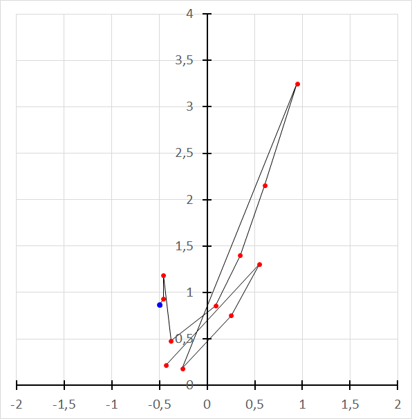
An example Newton fractal orbit.
The orbit elements resulting from applying a root-finding algorithm finally converge to one of the roots of the function. In the above example, that root is (-0.5, 0.866...) and the last orbit element which reached the root is marked blue.
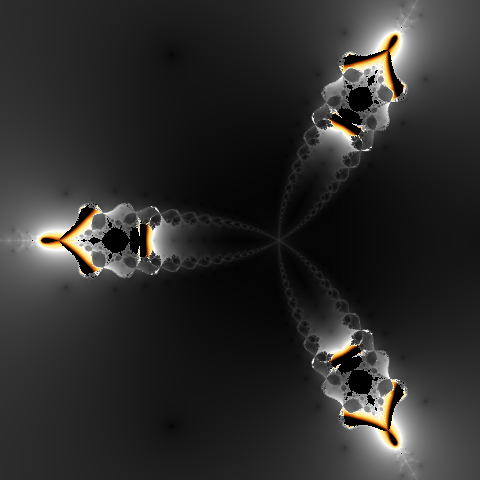
Root-finding fractals are often colored depending on which function root is found. They can also be colored depending on how many iteration steps it takes to find a root.
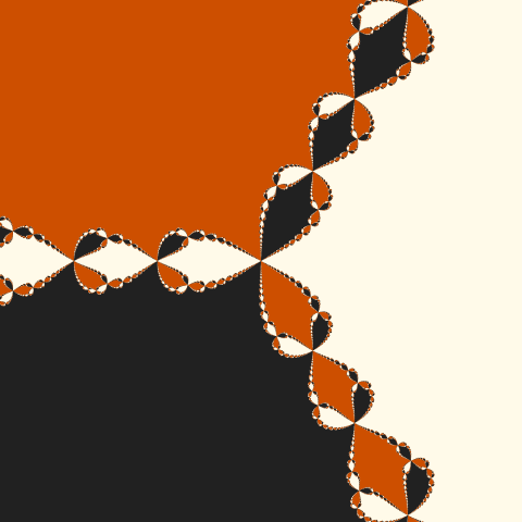
Newton fractal images using root found based coloring (on the left)
and orbit length based coloring (on the right).
The root is found when the next orbit value is equal to the previous one. In this case, we want to break the iteration. Considering floating-point errors, the escape condition can be as follows:
|zi - zi-1| ≤ bailout
where the bailout value should be reasonably low like 1e-7.
Actually the app's built-in CONVERGENCE escape condition is slightly more complex:
rad2(z - z[n-1]) / max(1, rad2 z) <= bailout
As with the DIVERGENCE condition, the squared absolute value |z|2 is used. Normalizing helps detect convergence to high value when the distance between subsequent orbit elements may be relatively high due to floating-point precision.
The bailout value used for the simple fractal definition is 1e-14. You may change it using the advanced definition.
As with the DIVERGENCE escape, we use a certain iteration limit, and treat the point as belonging to the fractal interior if no root is found within that number of steps.
There are some fractals based on root-finding idea, although they use disturbed formulas. The example is the Nova fractal which is the Newton fractal modified by adding c at each step and starting always from 1:
z0 = 1
zi+1 = zi - (zi3 - 1) / (3 zi2) + c
For those fractals, using the CONVERGENCE escape condition is a good choice and results in more impressive images than using the DIVERGENCE escape.
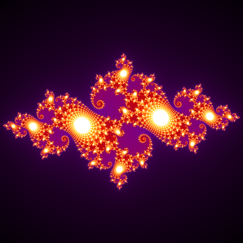
Nova fractal images using CONVERGENCE escape (on the left)
and DIVERGENCE escape (on the right).
Custom escape condition
Standard escape conditions (divergence, convergence) may not be the best choice for some fractal formulas. An example is the Collatz fractal defined as follows:
z0 = c
zi+1 = (1 + 4zi - (1 + 2zi) cos(Pi z)) / 4
Although it is possible to render a Collatz fractal image using standard divergence condition, a result can be more interesting when using the following custom escape condition:
|im(z)| > 4
Collatz fractal images rendered using BUILT-IN smooth and DIVERGENCE escape with bailout value 106 (on the left),
with bailout value 102 (in the middle) and with the custom escape condition and custom smooth (on the right).
The app allows you to define a custom escape condition by choosing CUSTOM escape in an advanced fractal definition.
Choosing the initial value
In most cases, you can simply use 0 as the initial value but there are some fractal formulas where it does not work. An example is the built-in Sinhbrot fractal using the following formula:
zi+1 = sinh(zi) c
Note that if the initial value of 0 were used, all the values would be 0 as sin(0)=0. So, in this case, the initial value is 1i.
Other examples are fractals where the current point value c is not used in the fractal formula (like the Newton fractal and the Collatz fractal described in the previous sections). In this case we have to use c for computing the initial value, otherwise all values would be the same.
Do not use 0 as the initial value when dividing by z is used in the formula. The examples are root-finding fractals like the Newton fractal or the Nova fractal. If 0 were used as the initial value, then when calculating the second value there would be a division by zero, and all the following values would be undefined.
Choosing different initial values may produce different images.
The Nova fractal with the initial value of 1 (on the left) and -0.795 (on the right).
Computing Julia sets
Let's consider a fractal type with the following definition:
z0 = A
zn+1 = F(zn, c)
where A is the orbit initial value and F(z, c) is a fractal formula.
The Julia set for this fractal will be computed as follows:
z0 = c
zn+1 = F(zn, complex(JuliaX, JuliaY))
The initial value is ignored and the current point c is used instead. The value of complex(JuliaX, JuliaY) is used instead of c in the fractal formula.
You may notice that for a fractal type where z0 = c and the value of c is not used in the fractal formula, computing the Julia set will give the same result as computing the original fractal. An example is the built-in Collatz fractal where the Julia mode has been disabled not to confuse a user. The built-in Newton fractal is another example. The Julia mode is also disabled for Lyapunov fractals where the results are completely unimpressive. On the other hand, there are built-in fractal types that are in the Julia Mode by default (like Phoenix), or that are available only in Julia Mode (like Violinbrot).
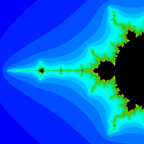
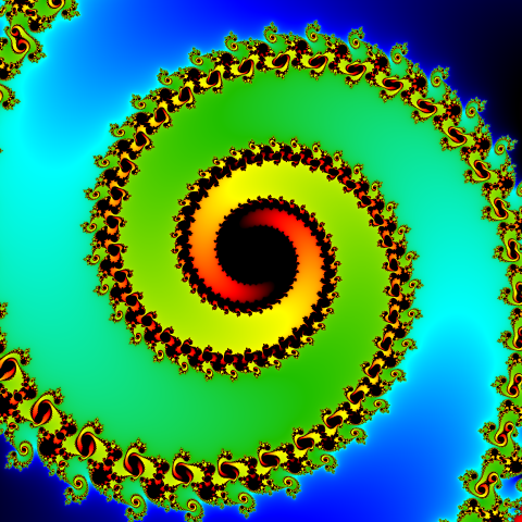
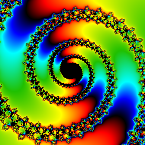
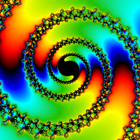
A common way for finding interesting Julia set image is to find a nice looking spot in some fractal and then use the coordinates as JuliaX/JuliaY values for rendering a Julia set image with the same formula. This is what the app does when you enter the Julia mode.
Julia set image usually shows a remarkable similarity to the spot from where you entered the Julia mode.

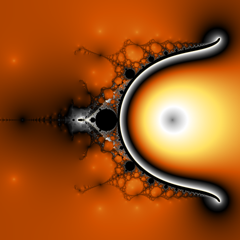
An example zoom-in of the Seahorse valley of the Mandelbrot Set (on the left)
and it's corresponding Julia set (on the right).
Coloring techniques
This chapter describes various techniques that can be used to color a fractal image.
The pixel color is determined based on the complex number sequence (called orbit) resulting from applying the fractal formula to the initial value corresponding to the pixel.
As it was mentioned earlier, the simplest method is the use of black for the pixels in which processing stops due to reaching the iteration limit (fractal interior) and white for the pixels where it stops because the escape condition is met (fractal exterior). In this way, you can visualize the shape of a fractal, but it is possible to get much more appealing images.
Iteration count coloring
One of the most used techniques is assigning a color to exterior pixels depending on the orbit length, i.e. how many iteration steps were performed before the escape condition was met.
First, we need a color scale (called palette). We set selected colors in specific places (from 0 to 1). The space in between will be filled with a smooth transition between the selected colors.
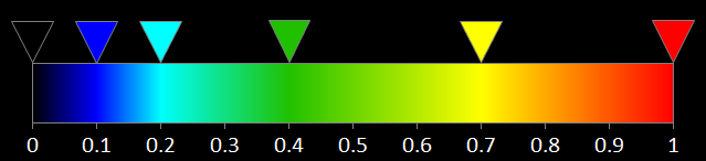
An example palette.
For a pixel with the orbit length equal n we use the palette color at position:
n / limit
where limit is the iteration limit. For example for the limit of 100 and the orbit length of 30 we use color at
30 / 100 = 0.3
Notice that 0.3 is halfway between 0.2 and 0.4 where we have certain colors in the example palette. This means that we should use the color halfway from cyan to green.

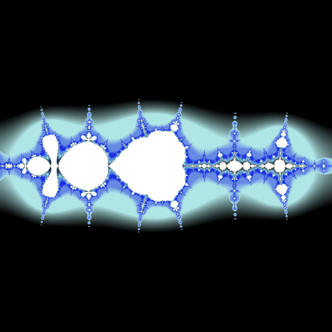
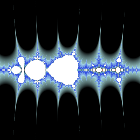
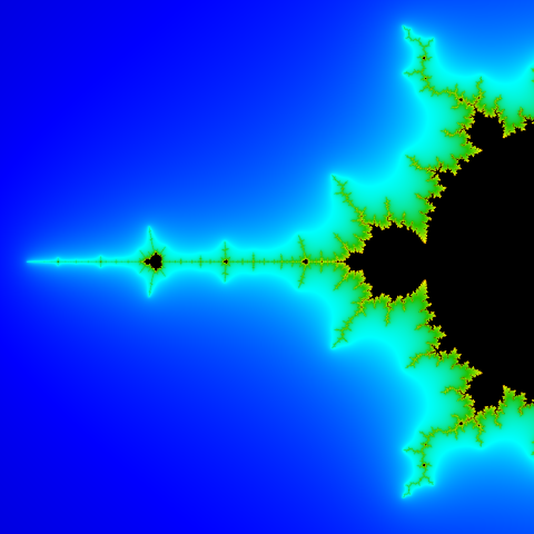
The Mandelbrot Set left antenna images using black and white coloring
and using iteration count coloring with the example palette.
In the image above we can clearly see the boundaries between areas with different iteration count values. These boundaries can be removed by using smoothing.
Color cycling
The technique described in the previous section uses one palette cycle to cover the entire iteration count range. However, many images can be made more appealing by using more palette cycles.
To achieve this, we need a palette that starts and ends with the same color, which allows a smooth transition to the next cycle.
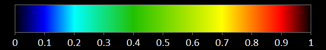
An example cyclic palette.
Next, we need to specify the iteration count range, which should be covered by one palette cycle. This number will be called palette length.
We can even get more control over the color, being able to shift the start of the cycle. This shift is a number in the range of [0, 1] and is called palette offset.
So, for a pixel with orbit length n, we calculate the position of the color on the palette as follows:
(n / length + offset) - floor(n / length + offset)
where length is the palette length, offset is the palette offset and the resulting color position is in the range of [0, 1]. Note, that we should use floating-point division.
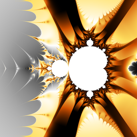
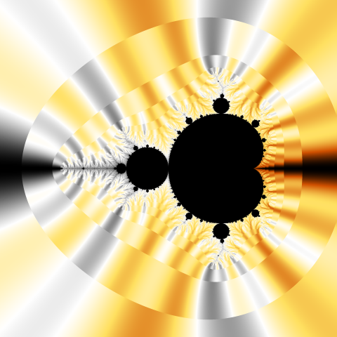
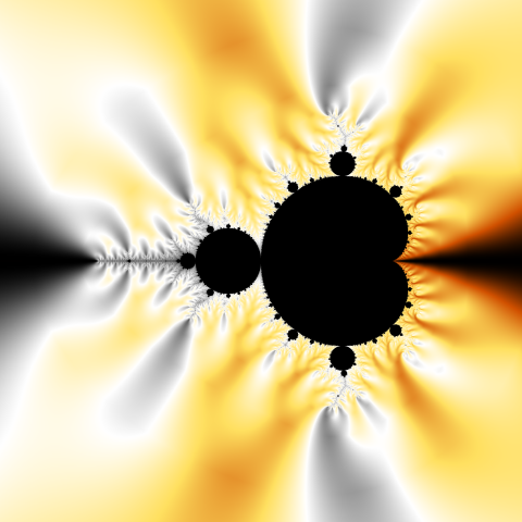
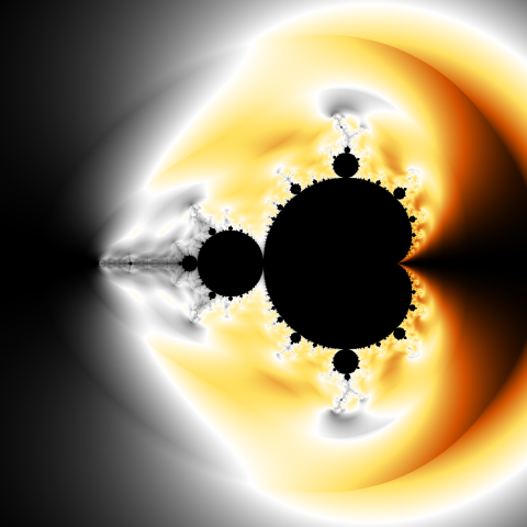
An example image using one palette cycle (on the left), using a shorter palette length (in the middle)
and with a palette offset applied (on the right).
Orbit based coloring
As it was mentioned earlier, the result of computing for a given coordinates is a sequence of n complex numbers:
z0, z1, z2, z2, ... , zn-1
which is called orbit. The iteration count coloring uses only the orbit length n, but we can get a lot of different patterns at the same fractal coordinates, using the values of the orbit elements to determine the color.
This can be done by applying a given formula to each orbit element, and then aggregating the results by calculating their average, minimum or maximum value. As the final result we get one floating-point number (called paint value) that can be used to determine the color position on the palette as described in the previous section:
(value / length + offset) - floor(value / length + offset)
where value is the paint value, length is the palette length and offset is the palette offset.
In many cases, it's a good idea to skip the first orbit element z0
as this is the initial value which may be the same for every pixel.
This is what the app does for simple definition paint modes, but in an
advanced paint mode definition
you can specify how many first elements to skip by assigning a value to the built-in variable
start in the initialization code section.
The following sections describe some uses of the orbit based coloring approach.
Orbit average coloring
There is a whole group of coloring methods based on average values and using different formulas. Some of them are quite well known and have their names like Stripe average coloring, Triangle inequality coloring or Curvature average coloring (these three are the app's built-in paint modes named Stripes, Veins and Branches, respectively).
Let's consider a simple method that calculates the average absolute value of the difference between the subsequent orbit elements:
|zi - zi-1|
An example images using different aggregation methods for |zi - zi-1| formula.
AVG(value) on the left and AVG(1 / (1 + value)) on the right (no smoothing applied).
The resulting image (the left picture above) is not very interesting because the last orbit elements with high values (just before exceeding the bailout) have a big impact on the average.
This issue can be solved by transforming the values before aggregation. For example applying:
1 / (1 + abs(value))
maps all the values to the range [0, 1] with the highest mapped to the values near 0 with a low impact on the average.
Other the app's built-in transformation methods are:
- atan(value)
- abs(atan(value))
- log(abs(value))
- abs(log(abs(value)))
Such a transformation is not always necessary. For example, Stripe average coloring method uses sin(arg(zi)) formula which gives the results from the limited range [-1, 1] and their average is not affected by the high values of the last elements of the orbit.
Example images using orbit average coloring with various paint formulas.
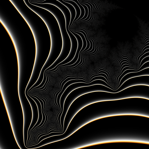
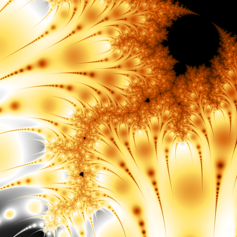
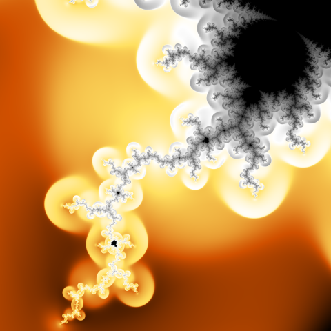
Orbit trap coloring
Another technique is the orbit trap method using the minimum distance between the orbit element and the selected geometric shape called trap. The most commonly used shapes are point, line (or several lines) and circle.
There is a visible similarity between the shape used as a trap and the patterns in the resulting image.
You can get more emphatic images using log(abs(value)) transformation before calculating the minimum value. This approach is used in the app's built-in paint modes: Straight wires (axis trap), Circle wires (circle trap) and Square wires (square trap).


Example Mandelbrot Set zoom images using different orbit trap based paint modes:
Straight wire, Circle wires, and Square wires (from left to right).
Instead of using the minimum orbit element distance to the trap, we may take the first (or the last) orbit element that falls inside the trap which can be a square, circle, or even more sophisticated shape (a star for example). Then we can determine the color based on the distance of that element from the trap edge and the element's position in the orbit.
This approach is used in the app's built-in paint modes with the names ending with "layers" (a single shape as the trap) or "pearls" (a ring of shapes as the trap). Those paint modes have the following common parameters controlling the way how the color is applied.
| Skip | The number of first orbit elements that are skipped. This allows to skip the first shape layers on the resulting image. |
| Range | The number of orbit elements that are processed after skipping the initial part of the orbit. Reducing the value allow to limit the number of shape layers visible. |
| Trap order | The order of shape layers. The value of 1 means, that the first orbit element falling inside the trap is taken, and this results in the largest shapes to be on the top. The value of -1 means, that the last orbit element falling inside the trap is taken, and brings the smallest shapes on the top. The intermediate values result in partially transparent layers. |
| Curvature | Impact of the orbit element distance from the trap edge on the final result. In other words, how much the color varies within a singe shape. |
| Color drift | Impact of the orbit element position in the sequence on the final result. In other words, how much the color varies between shape layers. |

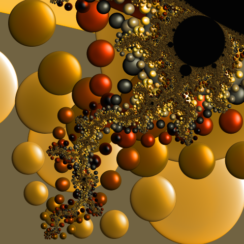
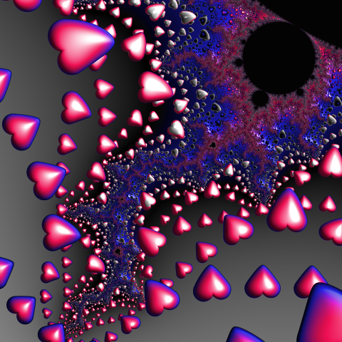
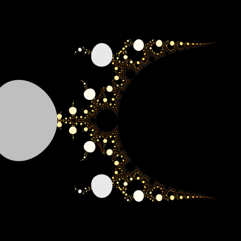
Example Mandelbrot Set zoom images using different orbit trap based paint modes:
Crescent layers, Round pearls, and Heart pearls (from left to right).
The two on the right have light applied.
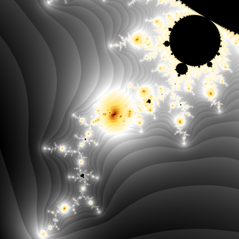
Photo coloring
The orbit trap technique can also be used for creating fractal images containing repeating photos. We use a rectangular trap (which is a photo). Then, instead of mapping the distance from the edge of the trap to a color from the palette, the color can be determined directly from the photo. We can simply map the coordinates of the orbit element that falls inside the trap to the photo coordinates, and take the color from that pixel of the photo (using interpolation to get a smooth result).
By using photos with transparent areas, we can get traps in any shape. When the orbit element is mapped to a transparent pixel in the photo, it does not count as hitting the trap.
Note that when applying the orbit trap method, the resulting image may contain shapes that are distored traps. Therefore, the photos in the resulting image can be distorted in various ways.
This technique is implemented by the app's special photo paint modes (with the names starting with "Photo"). The Skip, Range, and Trap order parameters work like in other orbit trap based paint modes.

An example result of applying the Photo pearls paint mode to a Mandelbrot set zoom.
Hybrid coloring
Experimenting with various painting formulas led me to a new coloring technique which I called hybrid coloring. It involves the iterative calculation of a given formula (as in the fractal calculation) using orbit elements as input. The result is a new sequence of complex numbers, based on which we can determine the color value using any of the previously described methods.
In this method, we mix two fractal formulas in some way. This is where the name "hybrid coloring" comes from.
The example is the app's built-in Hybrid 1 (Wings) paint mode. The sequence is defined as follows:
d1 = c
di+1 = sinh(di czi)
where zi is the orbit element and c is the current point. The paint value is calculated using the orbit average method:
AVG(1 / (1 + |di|2))
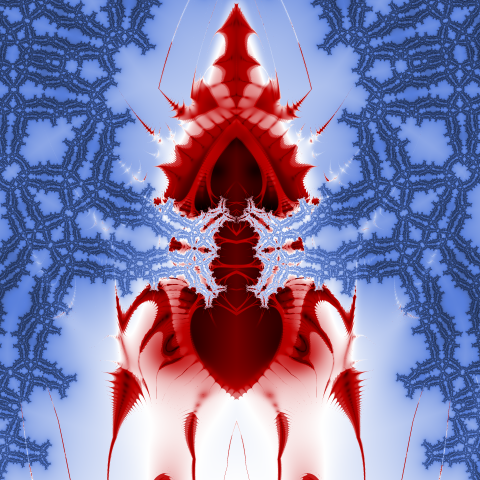
The patterns in the resulting image are quite unusual:
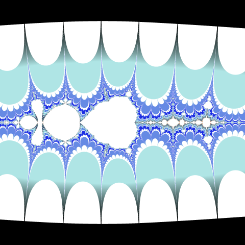
Mandelbrot Set image using the built-in Hybrid 1 (Wings) paint mode.
Images created using this approach often combine the shapes of the original fractal with the patterns resulting from the formula used to calculate the second sequence.


Example images using hybrid coloring.
Hybrid coloring methods may be created using advanced custom paint mode definition.
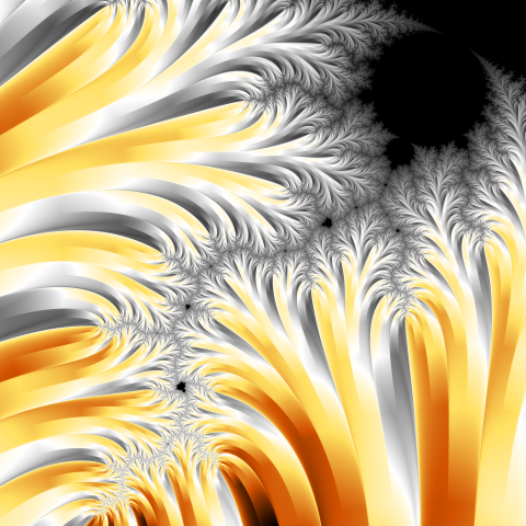
Smoothing
Fractal images may contain clearly visible boundaries between areas of different orbit lengths (iteration count values). The sharpness of these boundaries depends on the coloring method. For some methods, such as orbit trap, these borders are not visible.
Example images with no smoothing (on the top) and with smoothing (on the bottom).
These borders can be removed by using smoothing.
For each point, we need to calculate a smooth factor within a range of [0, 1].
This factor says how close the point is to the area of the next iteration count value.
The final paint value should be computed as follows:
smooth * value + (1 - smooth) * prev_value
where:
| smooth | a smooth factor value |
| value | a paint mode value for the whole orbit |
| prev_value | a paint mode value for the orbit with the last element excluded |
The smooth factor value is computed in the finalize code of a fractal type definition
and stored in the built-in variable smooth.
This value can be used in the finalize code of a paint mode definition for computing
a final paint mode value.
A proper method of computing the smooth factor value strongly depends on the escape condition. The app can compute the smooth factor for build-in escape types (DIVERGENCE, CONVERGENCE).
Most of the app's built-in fractal types and paint modes support smoothing.
Smoothing for DIVERGENCE escape
For polynomial fractal formulas (like z2+c) we can compute the smooth factor based on how close the last orbit element is to the bailout value. The formula for the smooth factor is as follows:
| log(log(bailout) / log(|zn-1|)) |
| log(exponent) |
where:
| bailout | the bailout value |
| zn-1 | the last orbit element (before exceeding the bailout value) |
| exponent | the highest power of z in the fractal formula |
Higher bailout values allow a better calculation of the smooth factor and smoother images. This is because for the last elements of the orbit holds:
zi+1 ≈ ziexponent
as other components of the fractal formula are very small relative to ziexponent. This means that we can use only zn-1 to estimate how close the point is to the area of the next iteration count value.
Example smooth images with bailout=100 (on the left) and bailout=2e+8 (on the right).
For many other fractal formulas, this approach can still be used after the empirical selection of the exponent value. If the formula contains division, it is worth using the difference between the highest power in the numerator and denominator.
The app stores the exponent value in the built-in variable exponent.
For simple definition custom fractals, the app estimates the exponent value
based on the fractal formula.
In an advanced definition, you should set the proper value in the initialization code section.
The following code snippet shows how the app computes the smooth factor for DIVERGENCE escape.
Note that because bailout variable holds squared bailout value, we must use the squared absolute value of the
last orbit element.
    R = rad2 z[n - 1];

    smooth = R > 1 ? log(log bailout / log R) / log exponent;

    smooth = max(0, min(1, smooth));
Smoothing for CONVERGENCE escape
For CONVERGENCE escape, the smooth factor can be computed based on the bailout value and the distances between the last elements of the orbit. The formula for the smooth factor is as follows:
| log(bailout) - log(|zn-1 - zn-2|) |
| log(|zn - zn-1|) - log(|zn-1 - zn-2|) |
where:
| bailout | the bailout value |
| zn-2, zn-1 | the last two elements of the orbit |
| zn | the last computed value (which does not belong to the orbit) |
The following code snippet shows how the app computes the smooth factor for CONVERGENCE escape. Note that the distances are normalized as was discussed earlier.
    R = rad2(z - z[n - 1]) / max(1, rad2 z);

    prev_R = rad2(z[n - 1] - z[n - 2]) / max(1, rad2(z[n - 1]));

    smooth = (log bailout - log prev_R) / (log R - log prev_R);

    smooth = max(0, min(1, smooth));